• This project explores the use of the NHiTS [5] neural network to forecast trajectories on the Lorenz Attractor. Given $2H$ points of input, the model is trained to predict the next $H$ points of the trajectory, where $H$ is usually 100 and $dt \approx 0.015$.
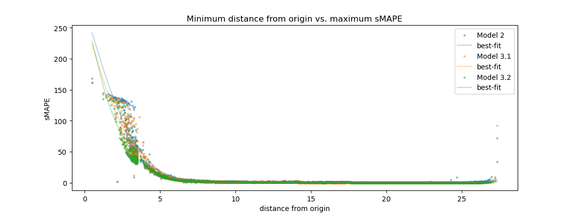
• The best performing models are able to predict trajectories in all areas of the attractor's subspace with high accuracy, except for trajectories that pass close to the saddle point at the origin (L2 distance $\lt \approx 5$). Trajectories in this region exhibit very high prediction error in the segments immediately following their transit past the origin, with the error increasing rapidly as the distance from the origin decreases.
• In 100% of test cases, trajectories that exhibit high prediction errors also have a local maximum Z coordinate in the range of $38.45$ to $38.6$. As temporal resolution of the model is increased, this value converges to approximately $38.55$, which is in near perfect agreement with certain limits implied by the Lorenz Map. Trajectories that meet this criteria have a roughly 60% chance of exhibiting a sMAPE prediction error greater than 5; otherwise the sMAPE error is guaranteed to remain below 5 at all times and in all other regions of the attractor subspace.

This project is inspired by several recent publications involving the use of deep learning to predict or control chaotic dynamical systems, in particular William Gilpin's paper, Model scale versus domain knowledge in statistical forecasting of chaotic systems [1]. Gilpin found that, given enough training data, generic neural architectures can match or exceed the performance of state-of-the-art domain-specific chaotic forecasting models such as reservoir computers and neural ODEs. I have recently become intrigued by the prospect of applying deep learning to prediction tasks involving chaotic systems, as I explore ways to contribute to the efforts to find technical solutions to climate change, and Gilpin's paper provided the impetus for me to begin this investigation. Along with [1], several other recent publications in related areas have been especially exciting to me, particularly the ones applying deep learning to tokamak control in nuclear fusion reactors (see e.g. [2], [3])¹.

My goal with this project is to get some hands-on experience with a chaotic system and probe deeper into Gilpin's findings by testing the limits of a generic (i.e. non-physics-informed) neural network's ability to model a single chaotic system (within the computational constraints imposed by my budget²). I'll start with what is probably the most well known chaotic system, the Lorenz Attractor. I will approach the problem more from the perspective of a generalist deep learning practioner than a dynamical systems expert, so I will be discovering many of the properties of the Lorenz System, and dynamical systems in general, as I go, often using the results of my experiments to guide my investigation³. What exactly makes the Lorenz Attractor chaotic? And what constraints will that impose on the ability of a deep neural network to model it?

Note: My intention is for this write-up to read more like a well-edited journal of my experiments and analyses than a proper research paper, so expect it to be a bit more verbose in some places than might seem necessary to convey the salient results.

Although the phenomon of sensitivity to initial conditions was first discovered by Henri Poincaré around the beginning of the 20th century in his research on the n-body problem, the birth of modern chaos theory is generally associated with the discovery of the Lorenz Attractor by Edward Lorenz et. al. in 1963 [4]. Lorenz developed the system as a simplified model of atmospheric convection while working on weather prediction.

The Lorenz system is comprised of three first-order ordinary differential equations representing the properties of convection and horizontal and vertical temperature in a two-dimensional fluid layer:

The Lorenz Attractor refers to a set of chaotic solutions to the system that constitute a strange attractor, that is, a system having a subspace towards which all trajectories tend to evolve (the attractor) and in which any given trajectory is so dense that its Hausdorff dimension exceeds its topological dimension (the strange part). The canonical parameterization of the Lorenz Attractor, which I will be using, is:

Other parameterizations of interest generally involve varying the $\rho$ parameter, for example, $\rho \lt 1$ in which the system is stable, and $\rho \approx 24.7$, at which a Hopf bifurcation occurs. But for this project, I will be focusing exclusively on the canonical parameterization.

For all trajectories in this project, I used Gilpin's dysts python module as a reference for the various parameters of the integration task for generating the training data.

The N-HiTS [5] forecasting network is known to produce state-of-the-art results, at the time of writing, for univariate time series prediction, with up to an order of magnitude lower computational requirement than some competitors. Given my limited budget and its strong performance reported in [1], it seemed like the natural starting point for a network architecture.

The architectural ideas in N-HiTS build on those of its predecessor, N-BEATS [6], a neural basis expansion network for time series prediction. The key ideas inherited from N-BEATS include the organization of fully connected layers into blocks that output basis expansions (linear projections of the preceding fully connected layer's output) and the use of both forecast and backcast predictions from each block. The forecast predictions from all blocks are summed together to produce the final output of the network, while the backcasts are subtracted from the input of the corresponding block to produce a residual connection as the input to the next block. The goal of the backcasts is to help the downstream blocks by "removing components of their input that are not helpful for forecasting" [6].

The novel ideas from N-HiTS enable the possiblity of modeling increasingly long time horizons while keeping computational complexity low. They include the use of pooling layers that downsample the inputs to each block and upsampling layers that map a compressed representation of the forecast to the output sample rate. In addition to the complexity savings, the compressed representations may induce a bias towards a temporal hierarchical modeling of the time series across the blocks that allows N-HiTS to exceed the performance of competing long-horizon forecasting models while requiring an order of magnitude lower computational complexity [5].

While Gilpin's experiments focus on testing 24 different time-series prediction models on over 130 different chaotic systems using a relatively narrow range of hyper parameters for tuning [1], my experiments aim to tune a single model, N-HiTS, on a single system, the Lorenz Attractor, to maximize its accuracy for a given, relatively long, fixed horizon (aka prediction window length). And more specifically, I aim not only to achieve a low average error on the test set but also to limit the worst-case error as much as possible, which will likely mean achieving a degree of predictive power over the most chaotic regions of the system. Is this a completely naive aspiration given what is known about chaotic systems? Maybe, but I'm not really sure yet, and either way this should be a great learning experience...

I begin with a horizon (prediction window), $H$, of 100 points, using a $dt$ of approximately $0.015$ seconds per point (the default from dysts) to sample the solution produced by the IVP solver. Importantly, note that this $dt$ is only the one used for sampling the solution after it is generated by the IVP solver. The actual $dt$ used internally by the IVP solver can vary dynamically, but the initial target value used by dysts is $\approx 1.8\mathrm{e}\text{-}\mathrm{4}$.

At this stage, it may also be worth mentioning one of the common metrics for measuring the average chaoticity of a system, the maximum Lyapunov exponent. As reported in dysts, the Lyapunov exponent, $\lambda_{max}$, for the Lorenz Attractor is approx. $0.8917$, and so the Lyapunov time is approx. $1.121s$.

This tells us that, on average, the distance between any two trajectories from the Lorenz Attractor are expected to diverge by a factor of $e$ after $1.121$ seconds. Note that with these parameters, the horizon covers a time period of about $\frac{4}{3}$ of the Lyapunov time. I can't say too much about the significance of this yet, other than to point out that because the Lyapunov exponent is positive, the distance between any two trajectories grows exponentially with time ¹, a defining feature of all chaotic systems.

The initial train and test sets are comprised of many trajectories with initial conditions all centered at approx. $[-9.79, -15.04, 20.53]$ and multiplied by a random perturbation uniformly sampled from the interval $[0.99,1.01]$.

The input to the N-HiTs model is a lookback window of the previous series values whose length is typically some multiple of the horizon window. I went with the default value from the N-HiTS paper of 5 times the horizon window length, or 500 points, making each training sample a total of 600 points. (Note that because N-HiTs is a univariate model, while the Lorenz System is three-dimensional, the data points must be flattened into one dimension. Therefore, the horizon window length is actually $3*100 = 300$, and each training sample's length is $3 * (500 + 100) = 1800$).

I choose, somewhat arbitrarily, to generate 10,000 points per series, and in order to increase data efficiency, I select each training sample by sliding the 600-point window along the series with a one-point stride. Each series, therefore, contributes $10,000 - 600 + 1 = 9401$ training samples. For the initial experiment, I generate 25 series with unique initial conditions, and train on 19 of them, and hold out 3 series for validation and 3 series for testing².

The full set of N-HiTS hyperparameters for the first model configuration is:

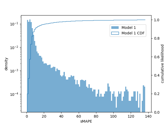
The model is optimized with MAE loss, consistent with the default loss from [5]. For evaluation, I use the symmetric mean absolute percentage error (sMAPE) as defined in [1]:

In this formulation, sMAPE is bound to the interval [0, 200]. The distribution of average window errors and its CDF on the test set are shown below. Note that the left y axis is log-scaled.

To gain a more intuitive understanding of the magnitude of these errors, we can plot individual window predictions against the references:

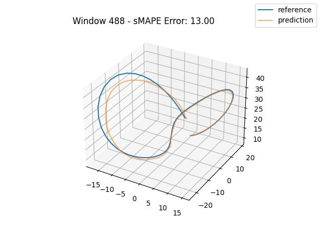
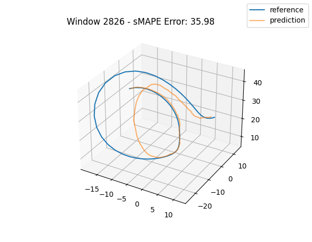
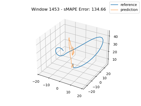
One interesting observation in all three graphs is that there appears to be a kind of "point of divergence" on the prediction before which the average error is very low and after which the error grows quickly. In the first graph, this point is about in the middle of the prediction, in the second it is maybe one third of the way into the prediction, and in the third it is near the beginning. If we look at the predictions of adjacent windows (see below animation), we see that the behavior at this point is consisent across the windows, indicating that there is something about the system's behavior in this region that is very difficult for this model to fit, regardless of its alignment within the prediction window.

For anyone familiar with dynamical systems theory, it won't be a surprise that this point coincides with one of the three critical points of the Lorenz system—in this case, the origin. And in this parameterization, the origin is known to be a saddle point comprised of the intersection of a stable 2D manifold and an unstable 1D manifold. "Stable" here means that trajectories near the critical point tend to move towards it even if they are perturbed slightly away from it by other forces, while "unstable" implies the opposite. (See [7] for some excellent visualizations of these manifolds.) Near the origin, the unstable manifold is a line that is approximately perpendicular to the Z axis and parallel to the lengthwise orientation of the Attractor, which is why the trajectories always diverge at the near-90-degree angles that we see in the animations as they approach the origin. And the (incredibly complex) topography of the stable 2D manifold determines towards which of the other two critical points a trajectory will be deflected [7]. In fact, we might technically say that the primary goal of the neural network is to learn the topography of the origin's stable 2D manifold; according to [7], this manifold defines a boundary across which trajectories can never pass, so we can confine the past and future path of any trajectory based on the boundaries of this manifold.

We can estimate how unstable the 1D manifold is by calculating the eigenvalues of the Jacobian matrix of the system at the origin and assuming the dynamics are approximately linear in this region (see Hartman-Grobman Theorem). When we do this, we get three eigenvalues, two of which have negative real components and are associated with the stable 2D manifold, and the third which has positive real component and is associated with the unstable 1D manifold. The dynamics along the manifolds near the origin can be approximated by the expression $f(t) = \exp(\lambda t)x_0$, where $\lambda$ equals the eigenvalue and $x_0$ is some initial point. For the Lorenz Attractor, the eigenvalue associated with the unstable manifold is $\approx 11.8$, so trajectories will be rapidly deflected away from the origin along the unstable manifold, as we see in the below animation:

Given all of this background, it is now unsurprising that the model is struggling to predict the behavior of the system near the origin. But we should also note that the model does quite well at predicting basically every other region of the system. If we can figure out a way to improve the predictions near the origin, then we should have a model with an overall very robust representation of the Lorenz Attractor. As this model and its training set are relatively modest in size, the next most obvious step to try is to significantly increase both the amount of training data and the model's capacity, and see if those changes alone are enough to resolve the weaknesses of Model 1.

For the next model, I increased the number of unique initial conditions from 25 to 10,000, and held out 100 for validation and 200 for testing, leaving 9,700 unique initial conditions, each of length 10,000 points, or about 150 seconds, in the training set. I also expanded the range of hyperparameters for tuning to include significantly larger models, both in depth and width. After tuning, I arrived at the following settings:

Note that Model 2 has roughly 32x the number of trainable parameters as Model 1. I've increased the depth (number of stacks, blocks per stack) and width (mlp layer size) of the network, and I've also significantly increased the amount of compression in the initial stacks. Because the network is much deeper, I also added layer normalization after each block to try to help reduce convergence time. Lastly, I increased the number of training steps and reduced the initial learning rate by an order of magnitude, and I modified the learning rate schedule to reduce by half whenever the validation loss does not decrease from the previous validation step.

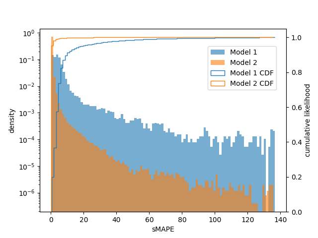
From the plot, we see a significant increase in the first bin and a reduction in every subsequent bin of the per-window error histogram relative to Model 1, so the larger dataset and new hyperparameter tunings have a definite and significant positive impact. 99% of windows from Model 2 have a sMAPE less than 6, compared to only 74% for Model 1, and 99.9% have a sMAPE less than 40, compared to 98% for Model 1.

There are, however, still a handful of windows with very large sMAPE errors. We can visualize these errors slightly differently to get a better sense of how they are distributed within and across the test series:

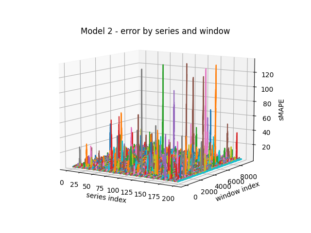
We see that very large errors occur quite rarely and briefly, with the predictions spending most of the time near the ground truth. Let's check the animation for one of the large spikes with a sMAPE greater than 100:

Not surprisingly, this trajectory passes very close to the origin, and we immediately see how similar this failure case is to the one from Model 1. Despite the average improvement across all error magnitudes, has the model's ability to predict the behavior near the unstable origin actually improved relative to Model 1? Let's check:

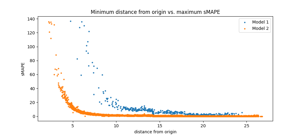
As we can clearly see from the plot, Model 2 is able to predict points that are closer to the origin more accurately than Model 1, so we have made some progress here. However, there is still a clear trend of an asymptotic increase in error as distance from the origin decreases. Could this be a fundamental property of the system, in which its predictability becomes exponentially more sensitive to error as the trajectories approach the origin? Or can we continue to make progress with some new model or training strategy?

With Model 2, we drastically increased both model capacity and dataset size, and we only achieved a marginal improvement on the most difficult trajectories. In this round of experiments, I will try a couple of new ideas that more specifically target these weak areas.

The first idea is to increase the percentage of trajectories in the dataset that pass very close to the origin so that the model sees more examples of these very tough cases during training. This turns out to be quite tricky task! Emperically, trajectories that pass very close to the origin are rare on the attractor, in the sense that just choosing a random intial condition from a point within the attractor volume is unlikely to produce a trajectory that passes very close to the origin in a relatively short amount of time. One idea is to choose a point that is already very close to the origin, and then use it as the initial condition to generate both a forward- and a backward-time solution. Then we can concatenate the two solutions together to produce a single solution with adequate time points before and after it approaches the origin. Sounds simple enough, except that when I attempted to produce the backwards solution, I inevitably ended up with a trajectory whose X coordinate grows in magnitude exponentially. In all of my attempts using the Radau solver with error tolerances approaching the limits of double precision, the X coordinate grew to the order of about $1\mathrm{e}{30}$ after about 0.5 seconds.

What's going on here? One possible explanation has to do with the finite volume that the attractor occupies. When we generate a forward solution starting with a point that is already on, or very close to, the attractor, we should be almost guaranteed to end up with a trajectory that remains on the attractor as $t \to \infty$, as this is the definition of an attractor after all. But the phase space is unbounded, and when we generate a backwards time solution, we are choosing a point on some aribtrary trajectory from the set of all trajectories in the phase space, including the ones that begin very far away from the attractor volume. The probability of randomly selecting a point that corresponds with a trajectory that has already been on the attractor for a sufficiently long period of time might be very low. However, this theory doesn't seem to explain why the X coordinate specifically would explode, while Y and Z remain on the attractor. And there are plenty of research papers that analyze backwards time solutions to the Lorenz Attractor (e.g.[7]), so clearly it is possible to generate backwards time solutions, I just have not been able to determine how. Possibly there is some issue with the numerical stability of the approaches I tried.

Failing to employ the backwards-time method, I will resort to cruder methods for generating a biased dataset. First I generate a very large number of trajectories (many more than I intend to use during training) using the same method as before for choosing the initial conditions. Then I sort these trajectories according to their minimum-L2 point and select the first N trajectories for inclusion in the dataset. I also take care to ensure that the distribution of trajectories across train, validation, and test sets is uniform with respect to these minimum points. When we plot the histogram of the windows from the dataset, grouping the windows based on their minimum points, we see that we've increased the number of windows in each of the groups with a distance from the origin $\lt{3}$ by a factor of about 10, while the total number of windows is the same as before:

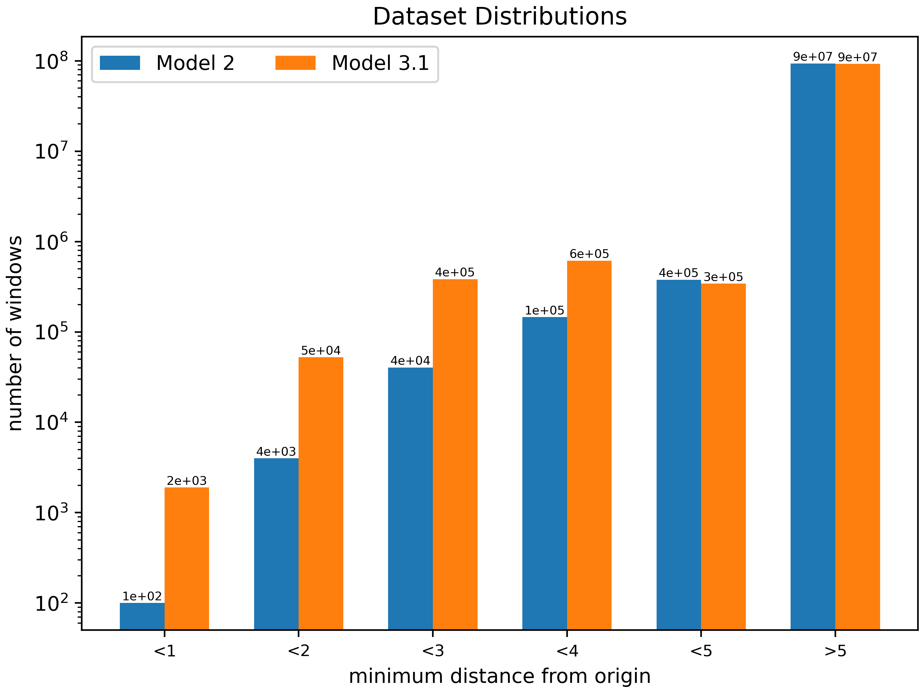
Still, with these 10x increases, the trajectories that pass within an L2 distance $\le{5}$ from the origin only comprise about 1.5% of the dataset (compared to 0.5% for the previous dataset). The other 98.5% is composed of what we already know to be easy cases for the model to predict.

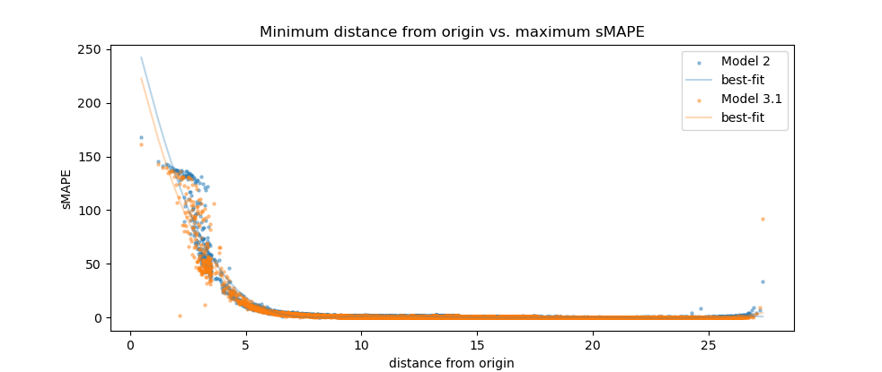
When we retrain the model using this dataset, we see a very slight improvement on the toughest cases. The error curve still increases asymptotically as the trajectory minima approach the origin, but it's also shifted slightly to the left:

Possibly we might continue to see incremental improvements if we continue to increase the percentage of the dataset that is comprised of these tough cases, but regardless, there seems to be a troubling trend emerging. The model does not appear to be extrapolating the dynamics of the system to this particular, small region of the attractor where data is sparse. For many real-world use cases, this behavior could be cost prohibitive; for example, in a nuclear fusion reactor, data collection is currently relatively expensive, and a severe failure can badly damage the reactor, leading to massive repair costs. Therefore, we should explore strategies other than increasing dataset size to address this problem first.

The next idea is to increase the temporal resolution of the model by using a smaller $dt$ to generate the data points. So far I've used a $dt$ of $\approx0.015$. Here I'll try reducing that by a factor of 5 to $\approx0.003$, and in order to keep the prediction task equally difficult, I'll also increase the horizon window by a factor of 5 to 500 so that the total amount of time being predicted is still $\approx1.5$ seconds. From tuning, I found that an input size of $2H$ performs just as well as an input size of $5H$, so I'll only increase the input size to 1000. I'll also use the same method as with 3.1 for generating a biased dataset, this time with 50,000 points per trajectory.

The new hyperparameters for Model 3.2 are:

A sidenote on the practicality of training this model: By increasing the input size and horizon length, we have significantly increased the memory requirement for training this model. Now in order to fit the model onto two GPUs with 16 GB of RAM each, I have to use Lightning's FSDP Strategy to distribute the model across both GPUs in order to get the per-GPU memory requirement to be just a hair under 16 GB. This also means that the model trains significantly more slowly, taking about 36 hours to converge, compared to about 16 hours for Model 2.

After retraining with $dt \approx 0.003$, we again see a very slight improvement over the previous models:

However, there doesn't appear to be any strong evidence that continuing to reduce $dt$ might lead to a fully stable model (i.e. one without an asymptotic error curve). And reducing it further will drastically increase the computational requirements of training, which are beyond my budget, so I must conclude this avenue of investigation here.

For the last experiment, I'll investigate the performance of the model when it is being used auto-regressively to generate a trajectory of arbitrary length given only the first $L$ samples of the reference trajectory, where $L$ is the input size of the model. This test can measure another aspect of the stability of the model: if the model produces small errors in its output that are then fed back to its input, do these errors compound in the feedback loop, leading to larger and larger errors in the output over time? Or does the model remain robust to these small input errors and continue to produce plausible trajectories indefinitely?

The term "plausible trajectory" needs some explanation, given that, in principle, the Lorenz Attractor is fully deterministic, so every trajectory is either a solution of the system or it isn't, i.e. there is no notion of the likelihood of a trajectory having been produced by the system or not. In practice, however, due to the finite precision of numerical computation, IVP solvers also make mistakes, injecting an element of stochasticity into the solutions they produce. The shadowing lemma tells us that, in spite of these errors, these "pseudo orbits" remain arbitrarily close to real trajectories so that the final solution can be said to faithfully represent the real trajectories of the system. However, some studies, e.g. [8], challenge this notion, demonstrating that in certain cases the statistics of the solver's outputs are distinct from those of true solutions of the system, and they can even imply a different parameterization of the underlying system. These are quite troubling implications for real-world applications, but I will delay further examination of this topic until the Discussion section.

In light of this, rather than evaluating the difference between the solver output and the model output, a more meaningful criterion may be to measure the similarity between certain statistics of their outputs. In [8], the following statistic of the Z coordinate is used to distinguish between what the authors refer to as "non-physical" solutions of the Lorenz Attractor and those that are typical true solutions:

Here's the distribution of this statistic for Model 3.2's autoregressive outputs and the Radau solver's outputs:

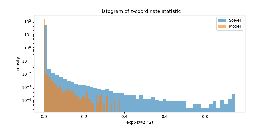
The general shape of the distributions is consistent, but clearly the solver outputs spend more time at Z coordinates very close to the origin as well as getting closer to the origin (minimum coordinate of $z \approx 0.4$ for the solver compared to $z \approx 1.35$ for the model). It's worth noting that the distributions of this metric for the other two coordinates, X and Y, match almost perfectly between the model and the solver.

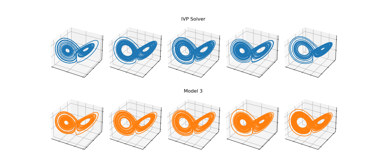
In we inspect them visually, we find that the vast majority of trajectories produced by the model look entirely plausible, possibily even indistinguishable to the human eye from the typical solver outputs:

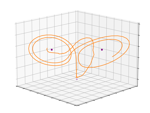
However, if we search for the model trajectories that pass closest to the origin, we find examples where the model output breaks down badly:

Another way to evaluate the autoregressive output of the model is to compare it with the output from a different IVP solver with similar error constraints. dysts uses the Radau solver by default, and this is what I used to generate the dataset. RK45 has similar error constraints to Radau, so let's compare the autoregressive output against Radau relative to RK45's output against Radau:

So we can say that the model is approximating the output of Radau more closely than another high-quality IVP solver. Ultimately, all three systems diverge chaotically from each other, but in the short term, Model 3 remains closer to Radau than RK45.

This project has probed the potential of the NHiTS neural architecture ([5]) to forecast the dynamics of the Lorenz Attractor, as estimated by the Radau IVP solver. Given $2H$ points of an initial trajectory, the neural model demonstrated the ability to predict the subsequent $H$ outputs of the Radau solver with very high accuracy in nearly all regions of the attractor's subspace. However, the dynamics in one region, the origin, proved to be too complex for the models tested here to capture. In all experiments, as trajectories approach the origin along the Z axis, the model's prediction error increases asymptotically. Significant efforts to augment the training data distribution in order to over-represent trajectories in this region imparted little or no improvement to the model's forecasting ability.

Similarly, when used autoregressively, the model demonstrated the potential to generate arbitrarily long trajectories that visually and statistically match the typical trajectories produced by the Radau solver for nearly all regions. But when the trajectories approach too close to the origin, the autoregressive output also breaks down, leading to solutions that visibly diverge from typical trajectories in obvious ways.

As already mentioned, it is well understood from dynamical systems theory that the saddle point at the origin of the Lorenz Attractor consists of a stable 2-d manifold and a highly unstable 1-d manifold. What this study suggests, and what is possibly not as well established, is that the predictability of the Lorenz Attractor largely depends on the trajectory's proximity to the origin. Trajectories on the attractor that remain sufficiently far from the origin are easily forecast by the model with high accuracy—including the transitions between each of the two lobes. But as trajectories approach the origin, and their velocities approach zero, they become asymptotically less predictable in the time period immediately before and after their transit past the origin (as the minimum distance to the origin decreases, this time period also increases). Fortunately, such trajectories appear to occur quite rarely on the attractor; in my experiments, when initial conditions are selected randomly from a point within the attractor volume, the trajectory has about a 1% chance of passing within a Euclidean distance of 3 or less from the origin within its first 150 seconds.

Trajectories that manage to pass so closely to the origin share other characteristics in common; for example, they are always nearly aligned with the Z axis as they approach the origin, and their velocities are dominated by the component in the negative Z direction. If we trace their paths back a bit farther, we notice a startling consistency among all trajectories with non-trivial sMAPE errors: the local maximum of the Z coordinate in the region of the trajectory just prior to approaching the origin converges to a value of approximately $38.55$. As the model's temporal resolution is increased, the bounds on this value become tighter. For Models 2 and 3, a trajectory having a local maximum Z coordinate in the range of $38.45$ to $38.6$ is a necessary condition for the model's sMAPE error to exceed 5 in the time period immediately following its transit past the origin¹.

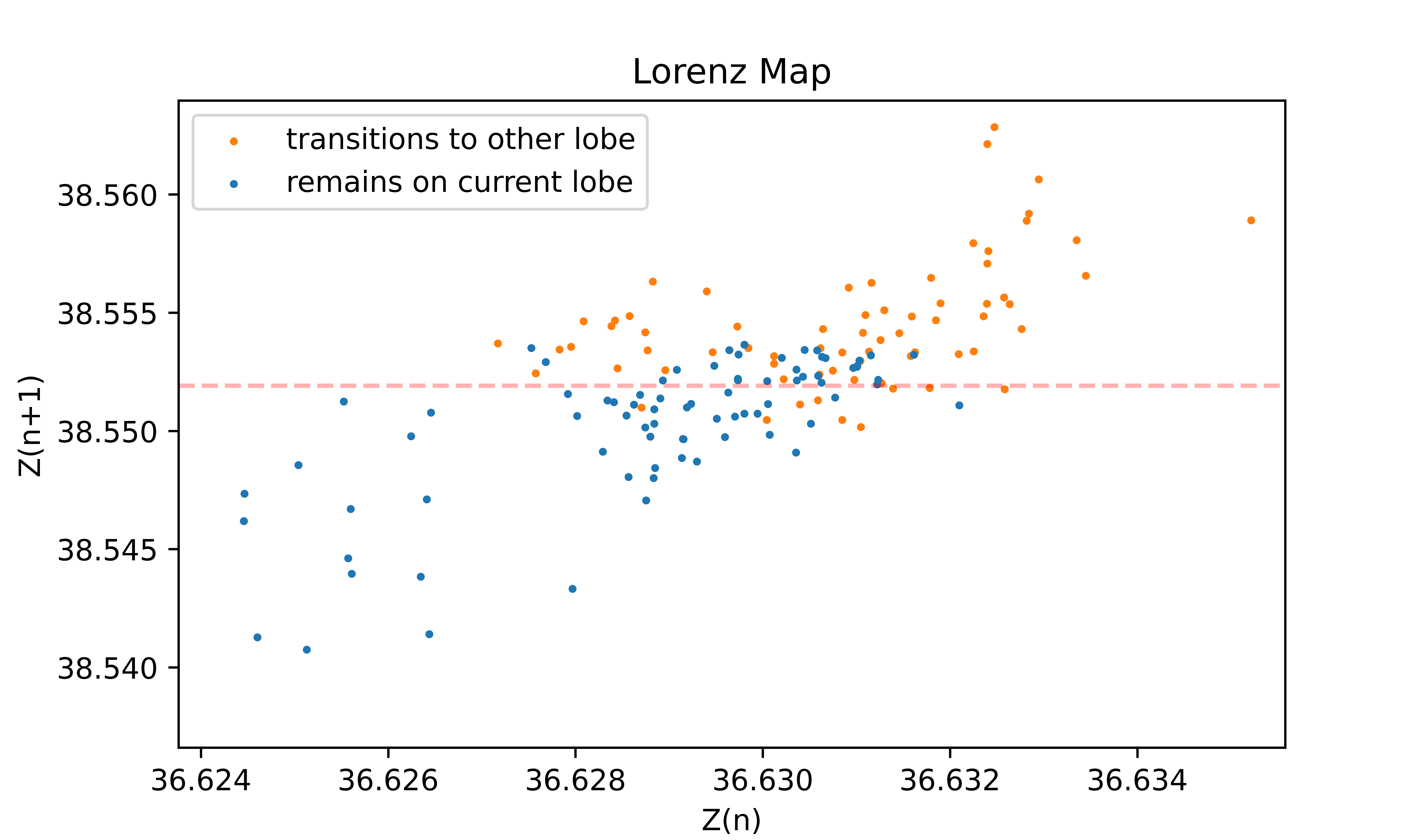
Lorenz himself also noticed peculiar patterns involving the local maximum Z coordinate and formulated the Lorenz Map to study the patterns. The map is shown below for Model 3.2's test set. The x coordinate at the transition point of the map (vertical dotted red line) corresponds almost perfectly with the limit suggested by the above error plots, about $38.55$. And the y coordinate that gives the best fit (minimum classification error) for separating trajectories that switch lobes at the end of the current orbital cycle from those that remain on the same lobe for at least another orbital cycle (horizontal dotted red line) also corresponds almost perfectly with this value. In other words, the most difficult trajectories for our models to predict are the ones that a) achieve the near-maximum observed Z coordinate (approximately 48) after passing by the origin, and b) straddle the threshold between transitioning from one lobe to the other or remaining on the current lobe for at least another orbital cycle.

This makes perfect sense. The trajectories that are the most difficult for the model to predict are the ones for which the tiniest perturbation can determine whether it transitions to the other lobe or remains on the current lobe. Finally, we have a concise way to describe the complexity of this prediction task. For the vast majority of trajectories, their transition probability is deterministic, either 100% or 0%, based solely on their Z coordinate local maximum. But there is a very narrow region of Z coordinates where the transition probability suddenly shifts to closer to 50%.

It would seem in one sense that the entire predictive complexity of the Lorenz Attractor is converging towards this Z value around $38.55$. As long as the local maximum Z coordinate of the trajectory does not pass through a narrow interval around this value, we can be certain (according to the statistics of all of the test sets in this study) that the model will continue to forecast the trajectory with a sMAPE error less than 5. If a trajectory does pass through this interval, then the model has a roughly 60% chance of exhibiting a sMAPE error greater than 5 in the period immediately following the peak, until the next local maximum Z coordinate is reached. How might we exploit this observation to improve predictability? If the system were augmented with a control input, then the target for that control could be to perturb the trajectories so that they avoid passing through this critical region around Z $\approx 38.55$. The results of this study suggest that this alone might make the dynamics of the Lorenz Attractor practically predictable.

Is this subtle inconsistency, in which the local Z maximum determines whether a transition will occur for all but a tiny range of values, an inherent property of the Lorenz Attractor, or could it somehow be a byproduct of the rounding error in the IVP solver? I don't know (please let me know if you do!), but if it's the former, then I would argue that this seems to impart a stochastic quality to the Lorenz Attractor that is incongruous with what we know to otherwise be a deterministic system. And if it's the latter, then we must ask how might the model would perform on a dataset in which the local Z maximum is linearly separable between these two groups, assuming we could somehow generate one? In this case, we would expect that the model's predictions for the toughest test cases, although they still might higher than average error, would at least not waiver indecisively between the two lobes, as they do now, but would instead commit to the correct lobe 100% of the time.

Sidenote: Upon discovering this apparent stochastic quality in the trajectories, I ran some follow-up experiments to see if I could generate such a dataset by using a smaller $dt$ parameter in the IVP solver. I tried values of $dt$ in the range $[1.8\mathrm{e}\text{-}\mathrm{4}, 1.8\mathrm{e}\text{-}\mathrm{5}]$. In all cases, the IVP solver eventually produced a trajectory that violated the linear separability requirement for the local Z maximum, and at $1.8\mathrm{e}\text{-}\mathrm{5}$, the numerical stability of the solver appeared to break down.

In closing, I will touch again on the implications of the shadowing lemma and research such as [8] for the feasibility of training models like these to predict real-world chaotic systems. It is well understood, and has been clearly demonstrated in this project, that IVP solvers produce imperfect solutions due to numerical rounding error. The models trained here, therefore, may be more accurately described as approximations of the IVP solver rather than of the true, mathematical idealization of the Lorenz Attractor represented by the ordinary differential equation introduced at the beginning of this study. Although technically deterministic, this rounding error introduces a kind of noise in the measurements of the system; similarly, any real-world dataset that is collected through environmental sensors will undoubtedly contain some amount of noise. While the shadowing lemma suggests that such noise may only marginally impact the correlation between the model and the chaotic system, [8] suggests the possibility that it can lead to highly divergent, non-physical solutions that may even be drawn from an entirely different system's distribution. The feasibility of modeling real-world chaotic systems may therefore hinge on the likelihood that a system emits "physical" shadowing solutions. If the likelihood is large enough, and especially if the system exhibits such narrow constraints on the conditions that lead to chaotically divergent trajectories as have been observed for the Z coordinate in this study, then effective control over chaotic dynamics may be tractable.

1. William Gilpin, Model scale versus domain knoweldge in statistical forecasting of chaotic systems, Phys. Rev. Res., vol. 5, pp. 043252, Dec, 2023, [link].
2. Seo, J., Kim, S., Jalalvand, A. et al., Avoiding fusion plasma tearing instability with deep reinforcement learning, Nature, 2024, [link].
3. Jonas Degrave, Federico Felici, Jonas Buchli, Michael Neunert, Brendan Tracey, Francesco Carpanese, Timo Ewalds, Roland Hafner, et. al., Magnetic control of tokamak plasmas through deep reinforcement learning, Nature, 2021, [link].
4. Oestreicher C., A history of chaos theory, Dialogues Clin Neurosci., 2007, [link].
5. Cristian Challu, Kin G. Olivares, Boris N. Oreshkin, Federico Garza, Max Mergenthaler-Canseco, Artur Dubrawski, N-HiTS: Neural Hierarchical Interpolation for Time Series Forecasting, arXiv:2201.12886, 2022, [link].
6. Boris N. Oreshkin, Dmitri Carpov, Nicolas Chapados, Yoshua Bengio, N-BEATS: Neural Basis Expansion Analaysis for Interpretable Time Series Forecasting, arXiv:1905.10437, 2019, [link].
7. Hinke M. Osinga, Understanding the geometry of dynamics: the stable manifold of the Lorenz system, Journal of the Royal Society of New Zealand, 2018, [link].
8. Nisha Chandramoorthy, QiQi Wang, On the probability of finding nonphysical solutions through shadowing, Journal of Computational Physics, 1 September 2021, [link].